How To Add Secondary Axis In Excel – 3 Easy Steps

How To Add Secondary Axis In Excel: Hi friends! If you’re here, it means you want to learn How To Add Secondary Axis In Excel. This guide will show you a simple and easy ways to do it.

In this article, we will learn how to add secondary vertical and horizontal axes in Excel. Adding a secondary axis in Excel is an easy and useful way to enhance your charts, especially when you have different types of data with varying ranges.

So, Let’s begin without wasting any time!

Why Add A Secondary Axis In Excel:

Adding a second axis might seem tricky, but it’s really about making your chart clearer and more useful. Here’s why you might want to use one:

1. Different types of data: If you’re showing numbers and percentages together, it can be very difficult. A second axis helps you display both clearly.
2. Big differences in numbers: When comparing very different values (like sales and taxes), one set might look too small or too big. A second axis gives each set its own space.
3. Different timeframes: If your data covers different time periods, a single axis can make it hard to see trends. A second axis helps show each timeline accurately.
4. Hidden relationships: Sometimes, data has connections that aren’t obvious. A second axis can help reveal these patterns.
5. Better storytelling: In reports or presentations, a second axis makes it easier to explain complex information and show how different things are related.

Here’s an example: Imagine you’re tracking how many products a factory makes each month and the percentage of defects. A standard chart might show blue columns for production and tiny orange columns for defects. With a second axis, both sets of data can stand out clearly.

How To Add Secondary Axis In Excel:

In older versions like Excel 2010, adding a second axis was a bit complicated. But in newer versions (Excel 2013 to 365), it’s much simpler. Here’s how to do it:

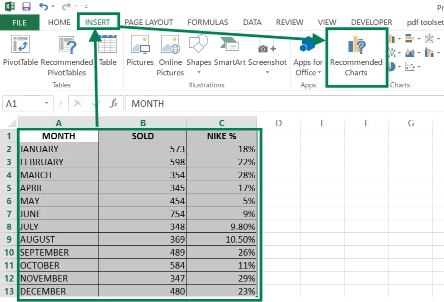
Step 1: Select Your Data: Choose the data you want to use for the chart, including the headers.

Step 2: Insert a Chart: Go to the Insert tab, click on Recommended Charts, and pick a chart type.

Step 3: Check for a Second Axis: If the recommended charts show one with a second axis, select it and click OK. If not, move to the next step.

Step 4: Choose a Combo Chart: In the All Charts tab, select Combo. For one set of data, pick Clustered Column, and for the other, choose Line. Check the Secondary Axis box for the line data, then click OK.

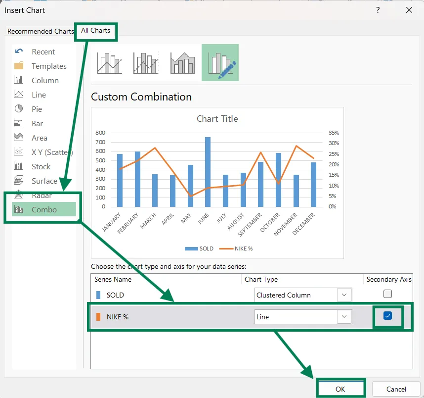
Done!: Your chart now has a second vertical axis.

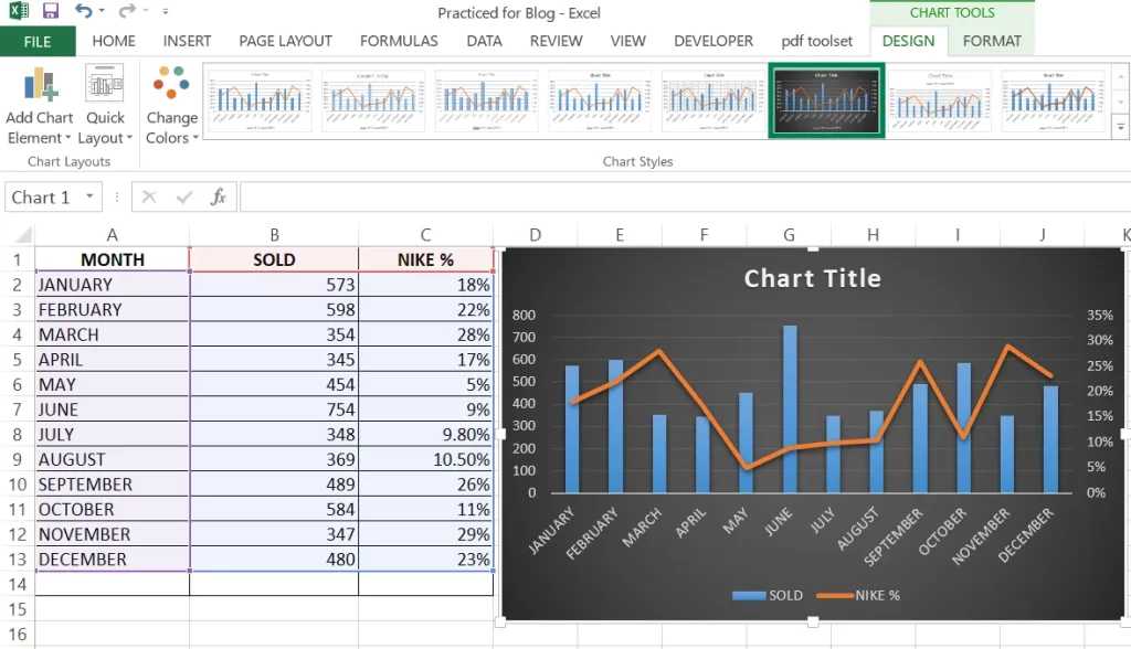
Tip: You can customize your chart further by adding titles or adjusting the design.

How To Add Second Y-Axis to an Existing Chart

If you already have a chart and want to add a second Y-axis:

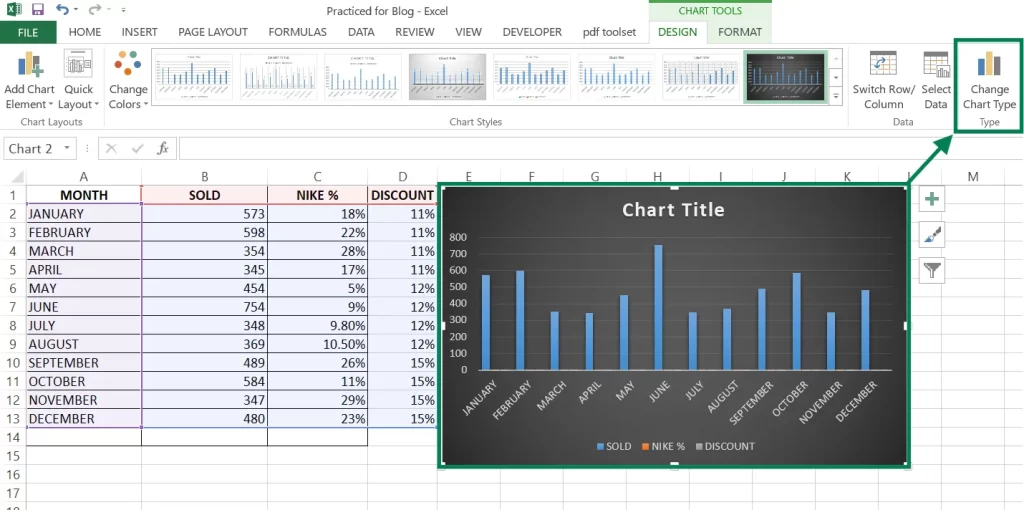
Step 1: Select the Chart: Click on the chart to activate the Chart Tools.

Step 2: Change Chart Type: Go to the Chart Design tab, click Change Chart Type, and select Combo.

Step 3: Pick the Right Chart: Choose Clustered Column – Line on Secondary Axis.

Step 4: Adjust the Axis: If needed, check the Secondary Axis box for the data series you want on the second axis.

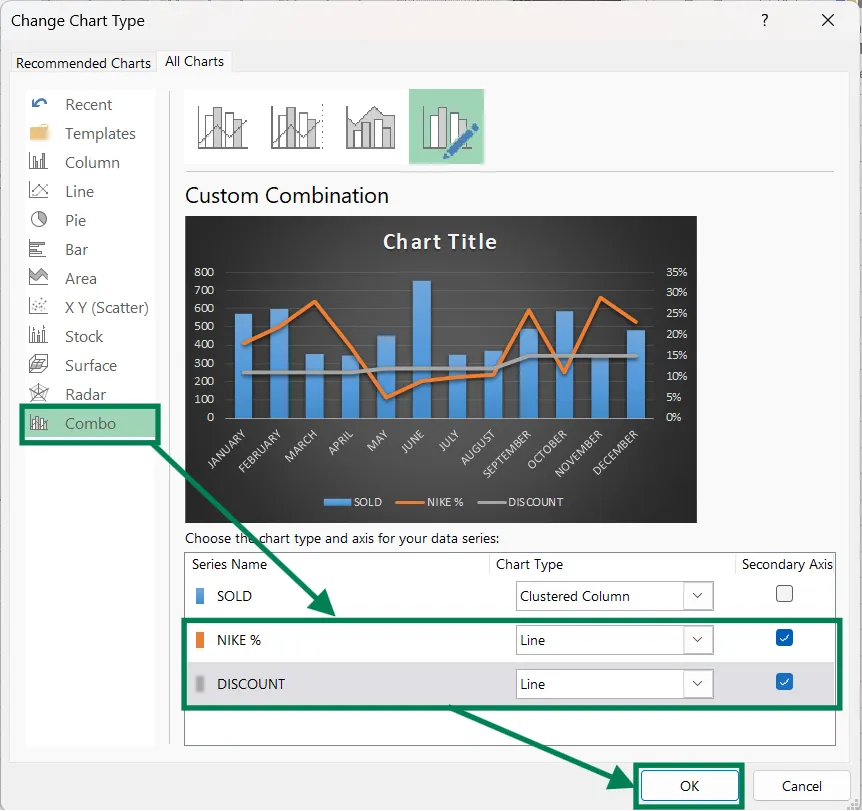
Step 5: Save Changes: Click OK, and your chart will now have a second Y-axis.

Also Read: Create Drop Down List In Excel

How To Add Second X-Axis in Excel

Adding a second horizontal X-axis is a bit trickier, but here’s how:

Step 1: Create a Blank Chart: Go to the Insert tab, and choose Scatter with Straight Lines without selecting any data.

Step 2: Add Data: Right-click the chart, click Select Data, and then Add to include your data series.

Step 3: Set Up Data Series: Name your first series (e.g., “Working”) and select the X and Y values. Repeat for the second series (e.g., “Defects”).

Step 4: Add a Second Axis: Double-click the series you want on the second axis, go to Format Data Series, and choose Secondary Axis.

Step 5: Switch to X-Axis: Click the Chart Elements button, uncheck Secondary Vertical, and check Secondary Horizontal.

Step 6: Adjust the Axis: If the second X-axis is in reverse order, click on it, go to Format Axis, and check Values in Reverse Order.

Step 7: Final Touches: Set the minimum, maximum, and units for each axis to make the chart look good.

How To Remove a Secondary Axis

To remove a secondary axis:

1. Delete It: Click on the secondary axis and press the Delete key.
2. Or Use the Menu: Click the Chart Elements button, go to Axis, and uncheck Secondary Axis.

That’s it! Your chart will go back to having a single axis.

Also Read: How To Create Search Box In Excel

Conclusion:

In conclusion, adding a secondary axis in Excel is an easy and powerful way to enhance your chart, especially when working with different types of data that have varying ranges. This guide helps you make your chart clearer and easier to read.

Simply follow the steps mentioned above: create a chart, select the data you want, and enable the secondary axis.

Thank you for reading this article to the end!